Exoplanet Hunting with Machine Learning and Kepler Data
In this post, our goal is to build a model that can predict the existence of an exoplanet (i.e. a planet that orbits a distant star system) given the light intensity readings from that star over time.
The dataset we’ll be using comes from NASA’s Kepler telescope currently in space. I’ll be taking you through the steps I followed to get from a low performing model to a high performing model.
The Kepler Telescope
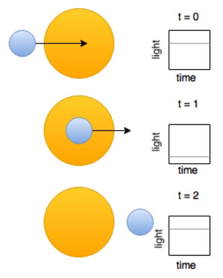
The Kepler telescope was launched by NASA in 2009, its mission is to discover Earth like planets orbiting other stars outside our solar system. Kaggle published a dataset containing clean observations/readings from Kepler in a challenge to find exoplanets (planets outside our solar system) orbiting other stars. Here’s how it works. Kepler observes many thousands of stars and records the light intensity (flux) that the stars emit. When a planet orbits a star, it slightly changes/lowers that light intensity. Over time, you can see a regular dimming of the star’s light (e.g. t=2 in the image below), and this is evidence that there might be a planet orbiting the star (candidate system). Further light studies can confirm the existence of an exoplanet on the candidate system.
The Kepler Telescope Dataset
The Kaggle / Kepler dataset is composed of a training set and a test set, with labels 1 for confirmed non-exoplanet and 2 for confirmed exoplanet.
Training Set:
- 5087 rows or observations.
- 3198 columns or features.
- Column 1 is the label vector. Columns 2–3198 are the flux values over time.
- 37 confirmed exoplanet-stars and 5050 non-exoplanet-stars.
Dev Set:
- 570 rows or observations.
- 3198 columns or features.
- Column 1 is the label vector. Columns 2–3198 are the flux values over time.
- 5 confirmed exoplanet-stars and 565 non-exoplanet-stars.
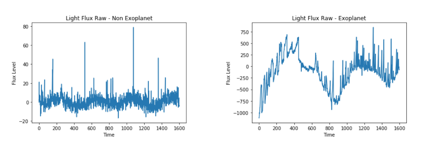
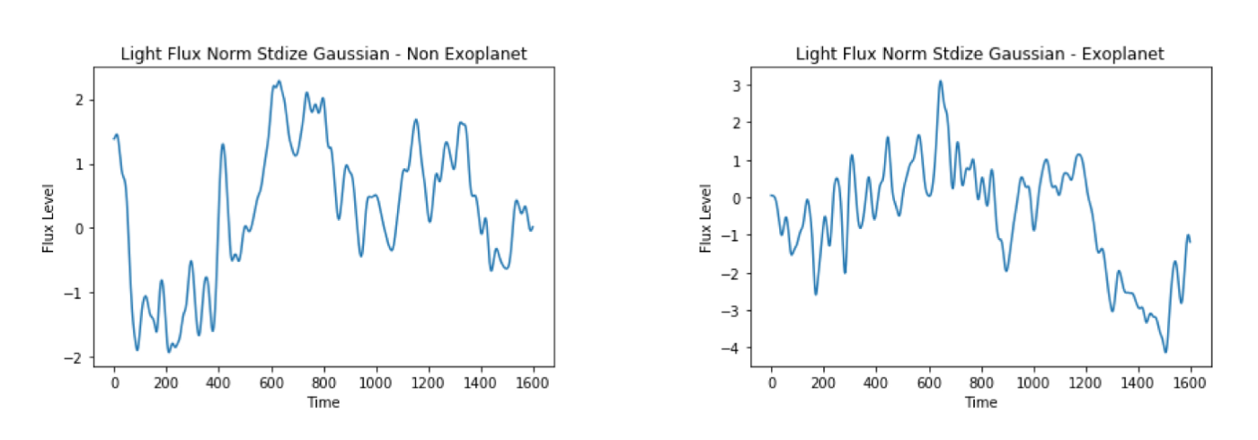
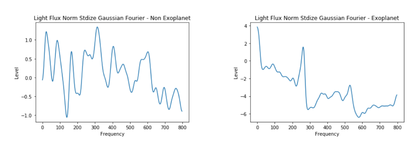
As an example, here is the light flux for an example with that is confirmed non-exoplanet (left) and an example that is confirmed exoplanet (right):
Goal -> Build a model that correctly predicts existence/non-existence of an Exoplanet
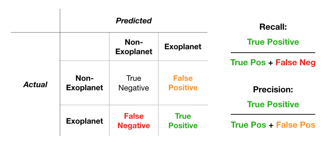
Due to the highly imbalanced dataset we are working with, we’ll be using Recall as our primary success metric and Precision as our secondary success metric (accuracy would be a bad metric because predicting non-exoplanet all across would get you very high accuracy).
Feature Engineering
Data Augmentation
First off, we have too few confirmed exoplanet examples in our data. There are several techniques that help overcome a highly imbalanced dataset and synthesize or create new examples. One we’ll use here is an algorithm called SMOTE (Synthetic Minority Over-sampling Technique). Instead of creating copies of examples, the algorithm essentially creates new examples by slightly modifying existing ones. This way we can have a balance of positive vs. negative examples in our training dataset.
Fourier Transform
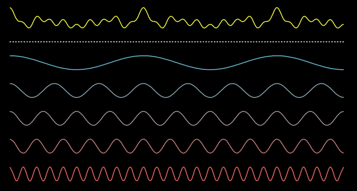
Anytime you are dealing with an intensity value over time, you can think of it as a signal or a mix of different frequencies jumbled up together. One idea to improve our model would be to ask ourselves, is there any difference between the frequencies that compose confirmed exoplanet light intensity signals vs. the frequencies that compose non-exoplanet signals. Fortunately, we can use the Fourier Transform to decompose these signals into its original frequencies, giving our model more rich/discriminative features.
Progression of Results
Our primary goal will be to maximize Recall on the dev set, but we’ll also maximize Precision as a secondary goal. For our model we’ll be using a Support Vector Machines model. In my testing, this model performed better than others I tested including several neural network architectures.
The graphs below are of examples index 150 (non-exoplanet) and index 4 (exoplanet).
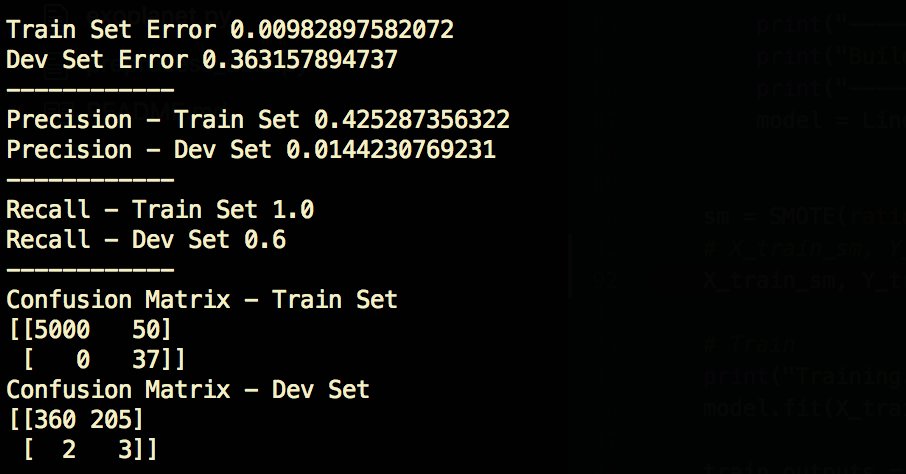
1. Unprocessed Data — Recall Train 100%, Dev 60%
Without any processing, we do well on the training set but our model doesn’t generalize well to the dev set. We can evidently diagnose our overfitting or high variance by looking at the big difference in train vs dev set errors. Since our model is already very simple, we’ll rely on feature engineering to make improvements.

2. SMOTE Data Augment— Recall Train 100%, Dev 60%
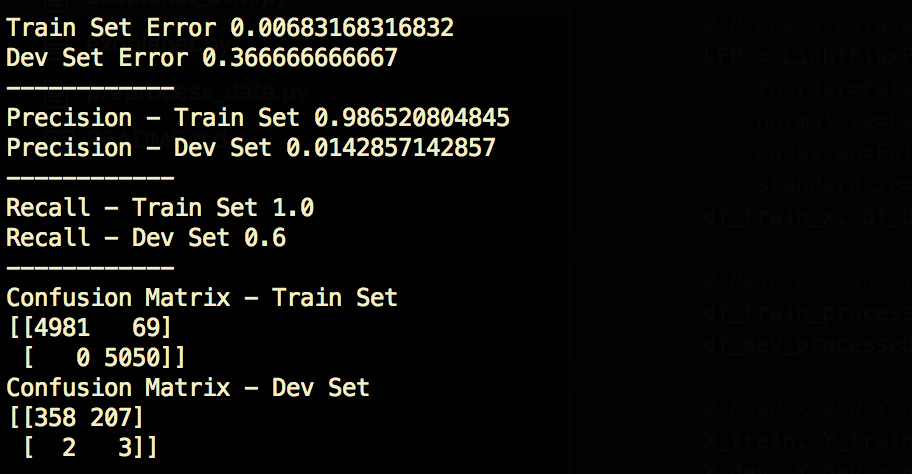
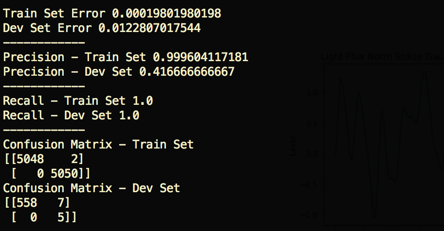
As a first step we will use the SMOTE technique to balance our training examples with the same amount of negative and positive examples. As you can see from the train confusion matrix below, we’ve increased our positive examples to be 5050, the same amount as negative examples. This will hopefully allow the model to better generalize to examples it hasn’t seen before. Notice how we are keeping the dev dataset untouched. This is important, you always want to test on real examples that you would expect ones you release the model to be used in the real world.
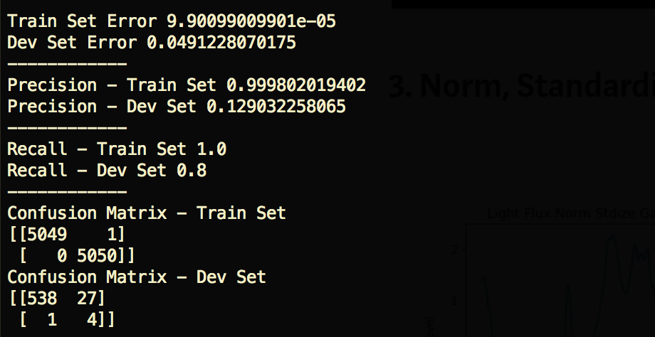
3. Norm, Standardize, and Gauss Filter— Recall Train 100%, Dev 80%
After normalizing, standardizing, and applying a Gaussian filter to our data, we can see an big improvement in recall and precision.
4. Fourier Transform — Recall Train 100%, Dev 100% — 42% Precision
This is where it gets more interesting. By applying the Fourier Transform, we’re essentially converting an intensity over time function to an intensity by frequency function. From looking at the chart, it seems that (at least for this particular example) there are some clear frequency spikes for the confirmed Exoplanet, giving our model richer and more discriminative features to train on.
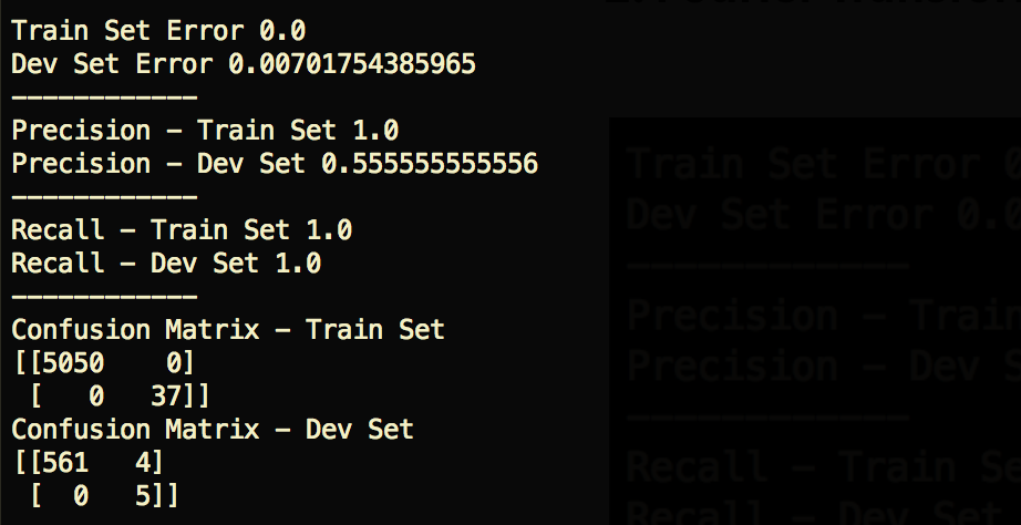
5. Without SMOTE — Recall Train 100%, Dev 100% — 55% Precision
I also tried the model without performing the SMOTE technique. Interestingly, it looks like, in this case, we can improve the precision of the model by not using SMOTE. I would be eager to test with/without SMOTE over a bigger dataset before coming to a conclusion on whether or not the technique should be used for this model.
Final Thoughts
It’s amazing we are able to gather light from distant stars, study this light that has been traveling for thousands of years, and make conclusions about what potential worlds these stars might harbor. Achieving a Recall of 1.0 and Precision of 0.55 on the dev set was not easy and required a lot of iteration on data pre processing and models.
This was one of the most fun projects/datasets that I’ve played around with and learned a lot in the process. As a next step, I’d be excited to try this model on new unexamined Kepler data to see if it can find new Exoplanets. Finally, it’d also be very interesting if NASA could provide datasets which include confirmed Exoplanets vs. Exoplanets in the Goldilocks Zone!
Kaggle (please upvote on top tight corner!): Kaggle Kernel
Full source code: https://github.com/gabrielgarza/exoplanet-deep-learning
Any comments / suggestions are welcome below ;)