Mask R-CNN for Ship Detection & Segmentation
In this post we’ll use Mask R-CNN to build a model that takes satellite images as input and outputs a bounding box and a mask that segments each ship instance in the image.
We’ll use the train and dev datasets provided by the Kaggle Airbus Challenge competition as well as the great Mask R-CNN implementation library by Matterport.
Link to code in Github: https://github.com/gabrielgarza/Mask_RCNN
Deep Learning
One of the most exciting applications of deep learning is the ability for machines to understand images. Fei-Fei Li has referred to this as giving machines the “ability to see”. There are four main classes of problems in detection and segmentation as described in the image (a) below .
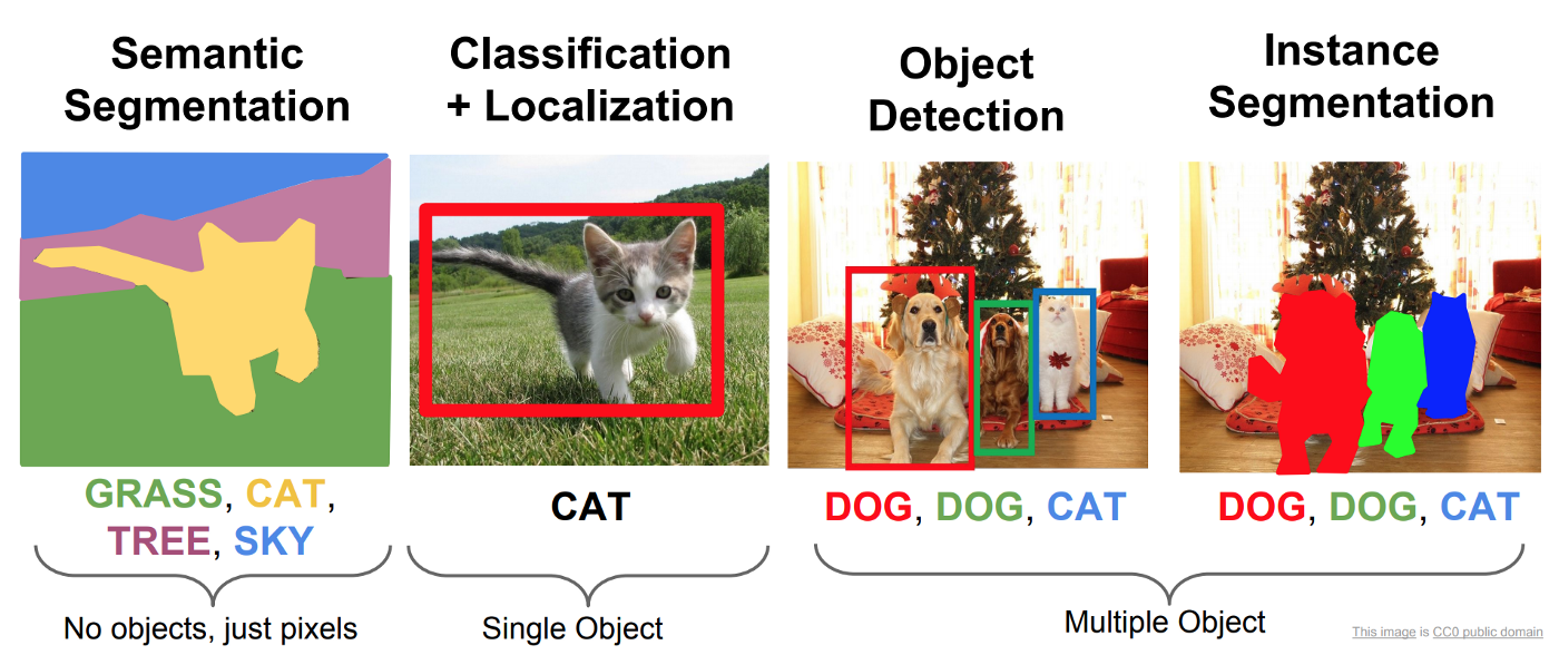
There are several approaches to Instance Segmentation, in this post we will use Mask R-CNN.
Mask R-CNN
Mask R-CNN is an extension over Faster R-CNN. Faster R-CNN predicts bounding boxes and Mask R-CNN essentially adds one more branch for predicting an object mask in parallel.
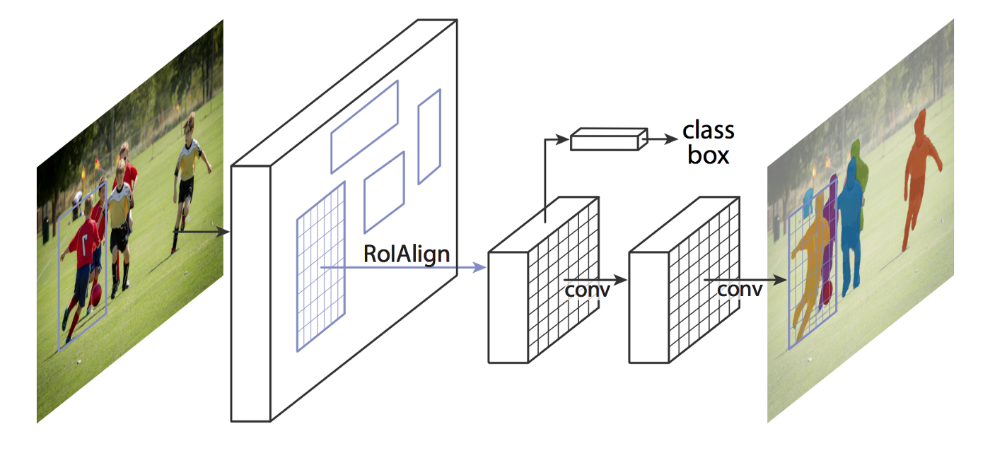
I’m not going to go into detail on how Mask R-CNN works but here are the general steps the approach follows:
- Backbone model: a standard convolutional neural network that serves as a feature extractor. For example, it will turn a1024x1024x3 image into a 32x32x2048 feature map that serves as input for the next layers.
- Region Proposal Network (RPN): Using regions defined with as many as 200K anchor boxes, the RPN scans each region and predicts whether or not an object is present. One of the great advantages of the RPN is that does not scan the actual image, the network scans the feature map, making it much faster.
- Region of Interest Classification and Bounding Box: In this step the algorithm takes the regions of interest proposed by the RPN as inputs and outputs a classification (softmax) and a bounding box (regressor).
- Segmentation Masks: In the final step, the algorithm the positive ROI regions are taken in as inputs and 28x28 pixel masks with float values are generated as outputs for the objects. During inference, these masks are scaled up.
Training and Inference with Mask R-CNN
Instead of replicating the entire algorithm based on the research paper, we’ll use the awesome Mask R-CNN library that Matterport built. We’ll have to A) generate our train and dev sets, B) do some wrangling to load the into the library, C) setup our training environment in AWS for training, D) use transfer learning to start training from the coco pre-trained weights, and E) tune our model to get good results.
Step 1: Download Kaggle Data and Generate Train and Dev Splits
The dataset provided by Kaggle consists of hundreds of thousands of images so the easiest thing is to download them directly to the AWS machine where we will be doing our training. Once we download them, we’ll have to split them into train and dev sets, which will be done at random through a python script.
I highly recommend using a spot instance to download the data from Kaggle using Kaggle’s API and upload that zipped data into an S3 bucket. You’ll later download that data from S3 and unzip it at training time.
Kaggle provides a csv file called train_ship_segmentations.csv with two columns: ImageId and EncodedPixels (run length encoding format). Assuming we have downloaded the images into the ./datasets/train_val/ path we can split and move the images into train and dev set folders with this code:
train_ship_segmentations_df = pd.read_csv(os.path.join("./datasets/train_val/train_ship_segmentations.csv"))

msk = np.random.rand(len(train_ship_segmentations_df)) < 0.8

train = train_ship_segmentations_df[msk]
test = train_ship_segmentations_df[~msk]

#  Move train set
for index, row in train.iterrows():
    image_id = row["ImageId"]
    old_path = "./datasets/train_val/{}".format(image_id)
    new_path = "./datasets/train/{}".format(image_id)
    if os.path.isfile(old_path):
        os.rename(old_path, new_path)

# Move dev set
for index, row in test.iterrows():
    image_id = row["ImageId"]
    old_path = "./datasets/train_val/{}".format(image_id)
    new_path = "./datasets/val/{}".format(image_id)
    if os.path.isfile(old_path):
        os.rename(old_path, new_path)
Step 2: Load data into the library
There is a specific convention the Mask R-CNN library follows for loading datasets. We need to create a class ShipDataset that will implement the main functions required:
# ship.py
class ShipDataset(utils.Dataset):

   def load_ship(self, dataset_dir, subset):

   def load_mask(self, image_id):

   def image_reference(self, image_id):
To convert a Run Length Encoded Mask to an image mask (boolean tensor) we use this function below rle_decode. This is used to generate the ground truth masks that we load into the library for training in our ShipDataset class.
def rle_decode(self, mask_rle, shape=(768, 768)):
    '''
    mask_rle: run-length as string formated (start length)
    shape: (height,width) of array to return
    Returns numpy array, 1 - mask, 0 - background
    '''
    if not isinstance(mask_rle, str):
        img = np.zeros(shape[0]*shape[1], dtype=np.uint8)
        return img.reshape(shape).T

    s = mask_rle.split()
    starts, lengths = [np.asarray(x, dtype=int) for x in (s[0:][::2], s[1:][::2])]
    starts -= 1
    ends = starts + lengths
    img = np.zeros(shape[0]*shape[1], dtype=np.uint8)
    for lo, hi in zip(starts, ends):
        img[lo:hi] = 1
    return img.reshape(shape).T
Step 3: Setup Training with P3 Spot Instances and AWS Batch
Given the large dataset we want to train with, we’ll need to use AWS GPU instances to get good results in a practical amount of time. P3 instances are quite expensive, but you using Spot Instances you can get a p3.2xlarge for around $0.9 / hr which represents about 70% savings. The key here is to be efficient and automate as much as we can in order to not waste any time/money in non-training tasks such as setting up the data, etc. To do that, we’ll use shell scripts and docker containers, and then use the awesome AWS Batch service to schedule our training.
The first thing I did is create a Deep Learning AMI configured for AWS Batch that uses nvidia-docker following this AWS Guide. The AMI ID is ami-073682d8e65240b76 and it is open to the community. This will allow us to train using docker containers with GPUs.
Next is creating a Dockerfile that has all of the dependencies we need as well as the shell scripts that will take care of downloading the data and run training.
FROM nvidia/cuda:9.0-cudnn7-devel-ubuntu16.04
MAINTAINER Gabriel Garza <garzagabriel@gmail.com>

# Essentials: developer tools, build tools, OpenBLAS
RUN apt-get update && apt-get install -y --no-install-recommends \
    apt-utils git curl vim unzip openssh-client wget \
    build-essential cmake \
    libopenblas-dev

#
# Python 3.5
#
# For convenience, alias (but don't sym-link) python & pip to python3 & pip3 as recommended in:
# http://askubuntu.com/questions/351318/changing-symlink-python-to-python3-causes-problems
RUN apt-get install -y --no-install-recommends python3.5 python3.5-dev python3-pip python3-tk && \
    pip3 install pip==9.0.3 --upgrade && \
    pip3 install --no-cache-dir --upgrade setuptools && \
    echo "alias python='python3'" >> /root/.bash_aliases && \
    echo "alias pip='pip3'" >> /root/.bash_aliases
# Pillow and it's dependencies
RUN apt-get install -y --no-install-recommends libjpeg-dev zlib1g-dev && \
    pip3 --no-cache-dir install Pillow
# Science libraries and other common packages
RUN pip3 --no-cache-dir install \
    numpy scipy sklearn scikit-image==0.13.1 pandas matplotlib Cython requests pandas imgaug

# Install AWS CLI
RUN pip3 --no-cache-dir install awscli --upgrade

#
# Jupyter Notebook
#
# Allow access from outside the container, and skip trying to open a browser.
# NOTE: disable authentication token for convenience. DON'T DO THIS ON A PUBLIC SERVER.
RUN pip3 --no-cache-dir install jupyter && \
    mkdir /root/.jupyter && \
    echo "c.NotebookApp.ip = '*'" \
         "\nc.NotebookApp.open_browser = False" \
         "\nc.NotebookApp.token = ''" \
         > /root/.jupyter/jupyter_notebook_config.py
EXPOSE 8888

#
# Tensorflow 1.6.0 - GPU
#
# Install TensorFlow
RUN pip3 --no-cache-dir install tensorflow-gpu

# Expose port for TensorBoard
EXPOSE 6006

#
# OpenCV 3.4.1
#
# Dependencies
RUN apt-get install -y --no-install-recommends \
    libjpeg8-dev libtiff5-dev libjasper-dev libpng12-dev \
    libavcodec-dev libavformat-dev libswscale-dev libv4l-dev libgtk2.0-dev \
    liblapacke-dev checkinstall
RUN pip3 install opencv-python

#
# Keras 2.1.5
#
RUN pip3 install --no-cache-dir --upgrade h5py pydot_ng keras

#
# PyCocoTools
#
# Using a fork of the original that has a fix for Python 3.
# I submitted a PR to the original repo (https://github.com/cocodataset/cocoapi/pull/50)
# but it doesn't seem to be active anymore.
RUN pip3 install --no-cache-dir git+https://github.com/waleedka/coco.git#subdirectory=PythonAPI

COPY setup_project_and_data.sh /home
COPY train.sh /home
COPY predict.sh /home

WORKDIR "/home"
Note the last three shell scripts copied into the container:
setup_project_and_data.sh -> clones our Mask R-CNN repo, downloads and unzips our data from S3, splits the data into train and dev sets, downloads the latest weights we have saved in S3
train.sh -> loads latest weights, runs the train command python3 ./ship.py train –dataset=./datasets –weights=last, uploads trained weights to S3 after training ends
predict.sh -> download the Kaggle Challenge test dataset (which is used to submit your entry to the challenge), generates predictions for each of the images, converts masks to run length encoding, and uploads the predictions CSV file to S3.
Step 4: Train the model using AWS Batch
The beauty of AWS Batch is that you can create a compute environment that uses a Spot Instance and it will run a job using your docker container, and then terminate your Spot Instance as soon as your job ends.
I won’t go into great detail here (might make this another post), but essentially you build your image, upload it into AWS ECR, then in AWS Batch you schedule your training or inference job to run with command bash predict.sh or bash train.sh and wait for it to finish (you can follow the progress by looking at the logs in AWS Watch). The resulting files (trained weights or predictions csv) are uploaded to S3 by our script. The first time we train, we pass in the coco argument (in train.sh)in order to use Transfer Learning and train our model on top of the already trained coco dataset:
python3 ./ship.py train --dataset=./datasets --weights=coco
Once we have finish our initial training run we’ll pass in the last argument to the train command so we start training where we left off:
python3 ./ship.py train --dataset=./datasets --weights=last
We can tune our model using the ShipConfig class and overwriting the default settings. Setting Non-Max Suppression to 0 was important to get rid of predicting overlapping ship masks (which the Kaggle challenge doesn’t allow).
class ShipConfig(Config):
    """Configuration for training on the toy  dataset.
    Derives from the base Config class and overrides some values.
    """
    # Give the configuration a recognizable name
    NAME = "ship"
# We use a GPU with 12GB memory, which can fit two images.
    # Adjust down if you use a smaller GPU.
    IMAGES_PER_GPU = 1
# Number of classes (including background)
    NUM_CLASSES = 1 + 1  # Background + ship
# Number of training steps per epoch
    STEPS_PER_EPOCH = 500
# Skip detections with < 95% confidence
    DETECTION_MIN_CONFIDENCE = 0.95
# Non-maximum suppression threshold for detection
    DETECTION_NMS_THRESHOLD = 0.0
IMAGE_MIN_DIM = 768
    IMAGE_MAX_DIM = 768
Step 5: Predict ship segmentations
To generate our predictions, all we have to do is run our container in AWS Batch with the bash predict.sh command. This will use the script inside generate_predictions.py, here’s a snippet of what inference looks like:
class InferenceConfig(config.__class__):
# Run detection on one image at a time
GPU_COUNT = 1
IMAGES_PER_GPU = 1
DETECTION_MIN_CONFIDENCE = 0.95
DETECTION_NMS_THRESHOLD = 0.0
IMAGE_MIN_DIM = 768
IMAGE_MAX_DIM = 768
RPN_ANCHOR_SCALES = (64, 96, 128, 256, 512)
DETECTION_MAX_INSTANCES = 20
# Create model object in inference mode.
config = InferenceConfig()
model = modellib.MaskRCNN(mode="inference", model_dir=MODEL_DIR, config=config)
# Instantiate dataset
dataset = ship.ShipDataset()
# Load weights
model.load_weights(os.path.join(ROOT_DIR, SHIP_WEIGHTS_PATH), by_name=True)
class_names = ['BG', 'ship']
# Run detection
# Load image ids (filenames) and run length encoded pixels
images_path = "datasets/test"
sample_sub_csv = "sample_submission.csv"
# images_path = "datasets/val"
# sample_sub_csv = "val_ship_segmentations.csv"
sample_submission_df = pd.read_csv(os.path.join(images_path,sample_sub_csv))
unique_image_ids = sample_submission_df.ImageId.unique()
out_pred_rows = []
count = 0
for image_id in unique_image_ids:
image_path = os.path.join(images_path, image_id)
if os.path.isfile(image_path):
count += 1
print("Step: ", count)
# Start counting prediction time
tic = time.clock()
image = skimage.io.imread(image_path)
results = model.detect([image], verbose=1)
r = results[0]
# First Image
re_encoded_to_rle_list = []
for i in np.arange(np.array(r['masks']).shape[-1]):
boolean_mask = r['masks'][:,:,i]
re_encoded_to_rle = dataset.rle_encode(boolean_mask)
re_encoded_to_rle_list.append(re_encoded_to_rle)
if len(re_encoded_to_rle_list) == 0:
out_pred_rows += [{'ImageId': image_id, 'EncodedPixels': None}]
print("Found Ship: ", "NO")
else:
for rle_mask in re_encoded_to_rle_list:
out_pred_rows += [{'ImageId': image_id, 'EncodedPixels': rle_mask}]
print("Found Ship: ", rle_mask)
toc = time.clock()
print("Prediction time: ",toc-tic)
submission_df = pd.DataFrame(out_pred_rows)[['ImageId', 'EncodedPixels']]
filename = "{}{:%Y%m%dT%H%M}.csv".format("./submissions/submission_", datetime.datetime.now())
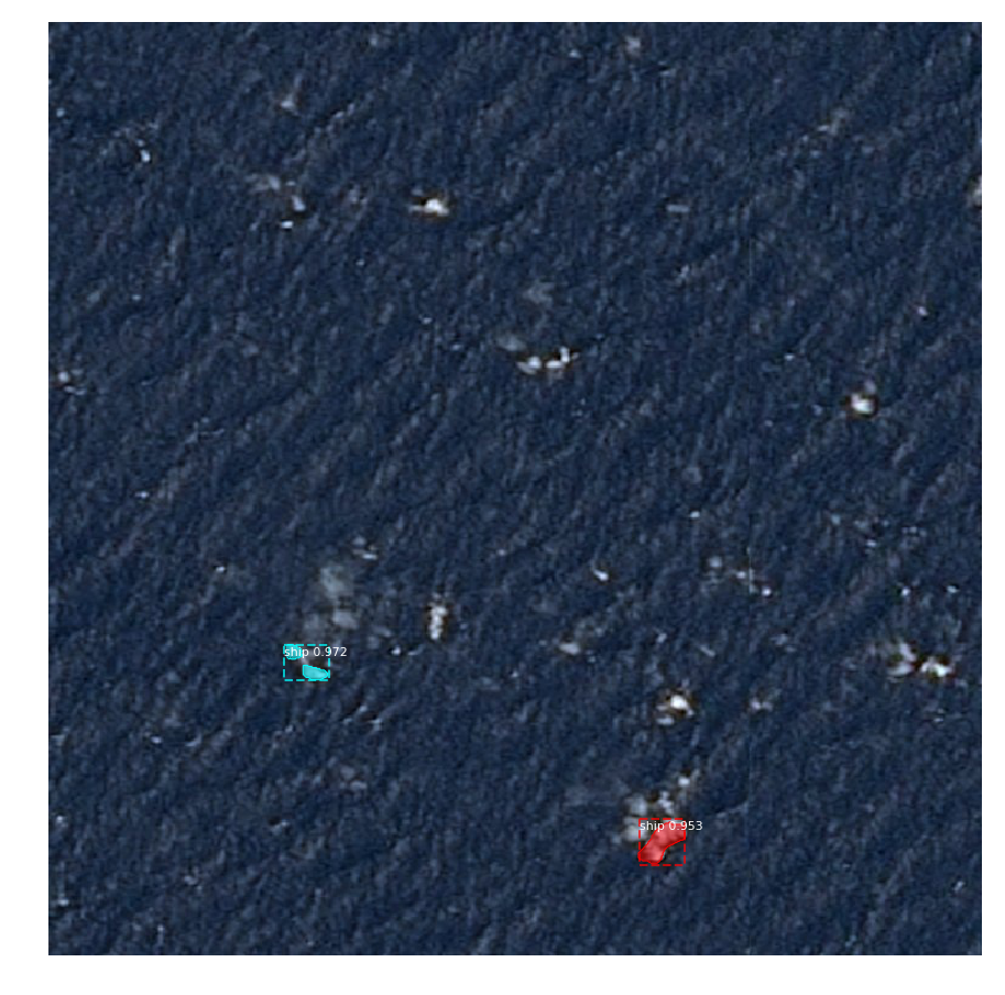
submission_df.to_csv(filename, index=False)I ran into several challenging cases, such as waves and clouds in the images, which the model initially thought were ships. To overcome this challenge, I modified the region proposal network’s anchor box sizes RPN_ANCHOR_SCALES to be smaller, this dramatically improved results as the model no longer predicted small waves to be ships.
Results
You can get decent results after about 30 epochs (defined in ship.py). I trained for 160 epochs and was able to get to 80.5% accuracy in my Kaggle submission.
I’ve included a Jupyter Notebook called inspect_shyp_model.ipynb that allows you to run the model and make predictions on any image locally on your computer.
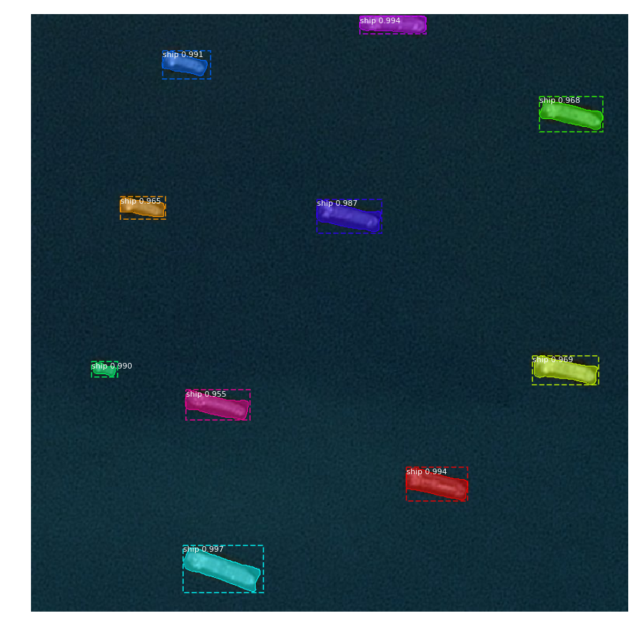
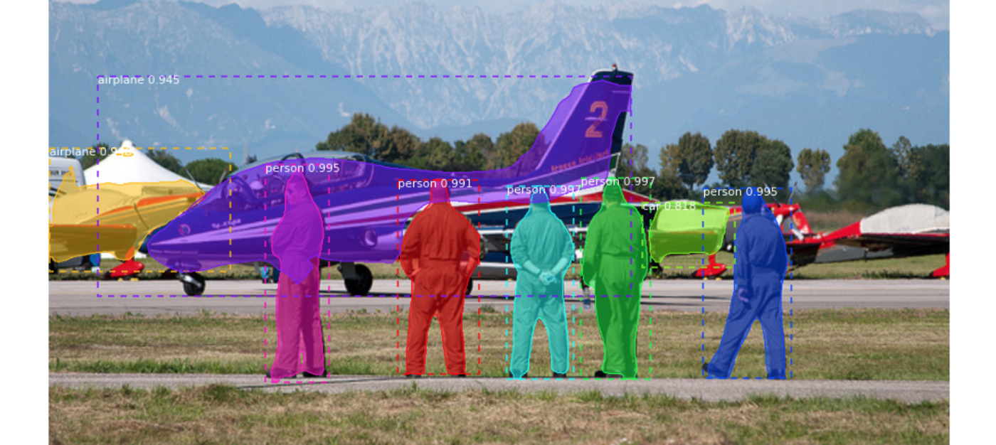
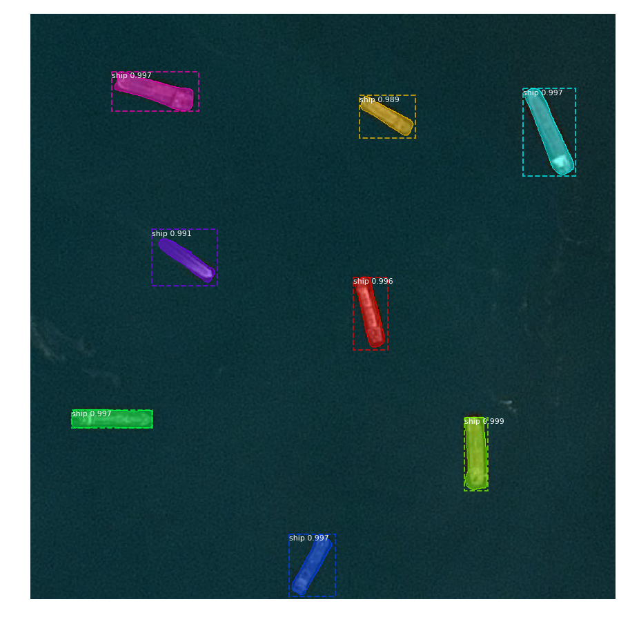
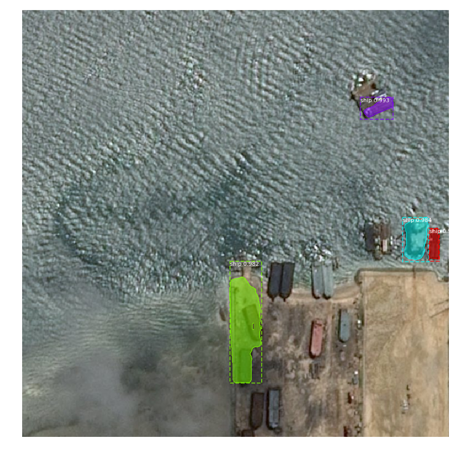
Here are some of example images with predicted probabilities of the instance being a ship, segmentation masks, and bounding boxes overlaid on top:
Mask R-CNN model predicting 8/8 ships with masks:
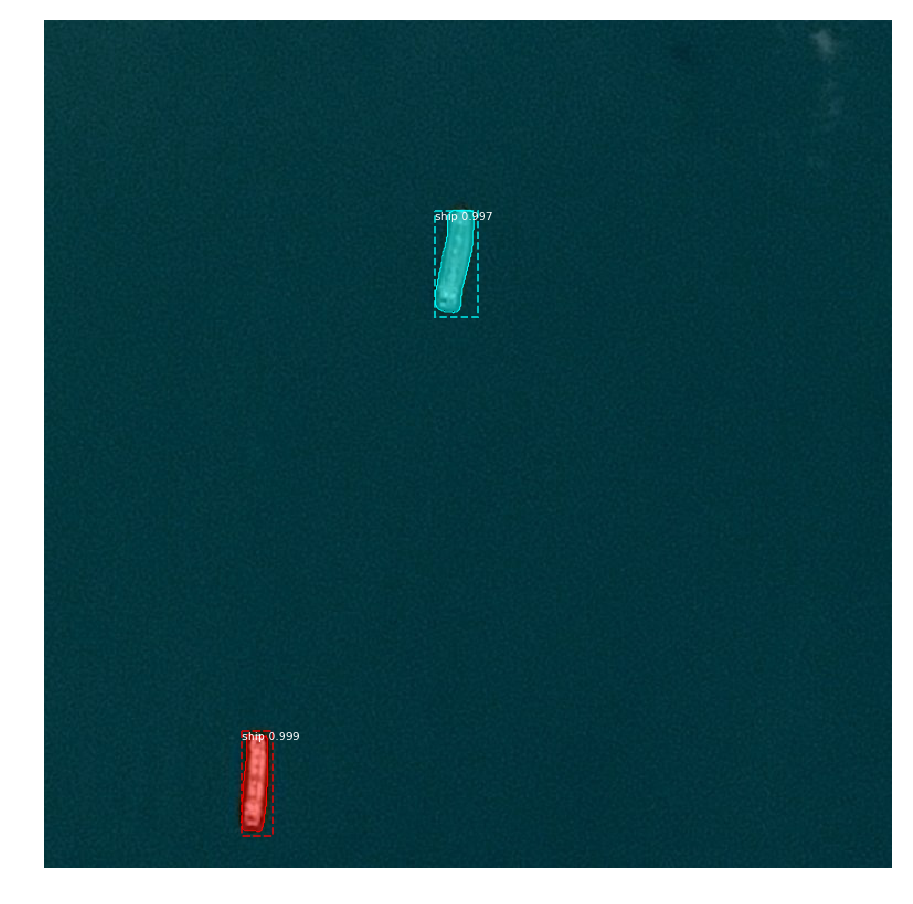
Model predicting 2/2 ships:
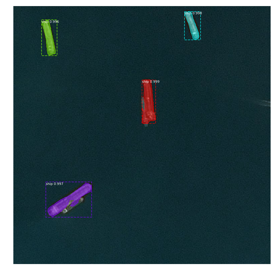
Model having some issues with ships that are right next to each other:
Waves generate false positives for the model. Would need to further train/tune to overcome completely:
Difficult image with some docked ships and some ships located on land.
Conclusion
Overall, I learned a lot on how Mask R-CNN works and how powerful it is. The possibilities are endless in terms of how this technology can be applied and it is exciting to think about how giving machines the “ability to see” can help make the world better.
Github Repo: https://github.com/gabrielgarza/Mask_RCNN